Machine Learning: R’s Statistical Approach

machine-learning

statistics

modeling

How R’s statistical foundation provides unique advantages for machine learning compared to Python’s engineering-focused approach

Published

June 19, 2025

1 Introduction

While Python dominates in deep learning and engineering-focused machine learning, R provides unique advantages through its statistical foundation. R’s approach to machine learning emphasizes interpretability, statistical rigor, and research-grade implementations that complement Python’s strengths.

2 R’s Statistical ML Foundation

2.1 Built on Statistical Theory

R’s machine learning is grounded in statistical theory:

Code

# R's ML approach emphasizes:
# - Statistical interpretability
# - Model diagnostics
# - Uncertainty quantification
# - Research reproducibility
# - Academic rigor

2.2 Research-Grade Implementations

R provides peer-reviewed machine learning packages:

Code

# R's ML packages are:
# - Peer-reviewed
# - Published in statistical journals
# - Used in academic research
# - Well-documented
# - Statistically validated

3 Statistical Learning with R

3.1 Linear and Generalized Linear Models

R excels in statistical learning:

Code

library(stats)
library(MASS)

# Linear models with comprehensive diagnostics
lm_model <- lm(mpg ~ wt + cyl + hp, data = mtcars)
summary(lm_model)


Call:
lm(formula = mpg ~ wt + cyl + hp, data = mtcars)

Residuals:
    Min      1Q  Median      3Q     Max 
-3.9290 -1.5598 -0.5311  1.1850  5.8986 

Coefficients:
            Estimate Std. Error t value Pr(>|t|)    
(Intercept) 38.75179    1.78686  21.687  < 2e-16 ***
wt          -3.16697    0.74058  -4.276 0.000199 ***
cyl         -0.94162    0.55092  -1.709 0.098480 .  
hp          -0.01804    0.01188  -1.519 0.140015    
---
Signif. codes:  0 '***' 0.001 '**' 0.01 '*' 0.05 '.' 0.1 ' ' 1

Residual standard error: 2.512 on 28 degrees of freedom
Multiple R-squared:  0.8431,    Adjusted R-squared:  0.8263 
F-statistic: 50.17 on 3 and 28 DF,  p-value: 2.184e-11

Code

# Model diagnostics
par(mfrow = c(2, 2))
plot(lm_model)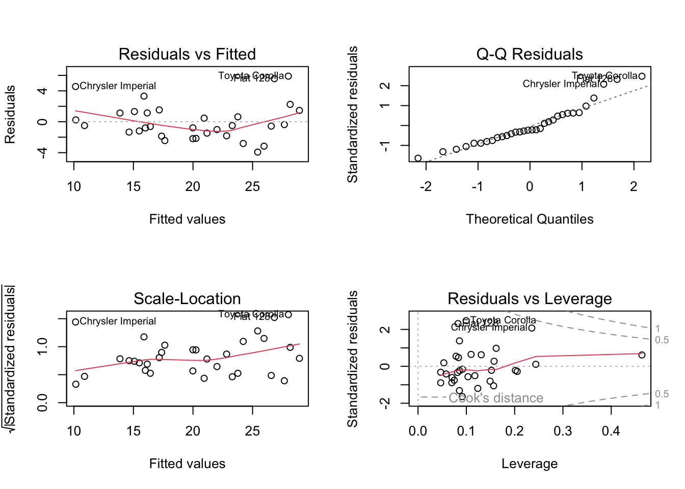

Code

# Stepwise selection
step_model <- stepAIC(lm_model, direction = "both")

Start:  AIC=62.66
mpg ~ wt + cyl + hp

       Df Sum of Sq    RSS    AIC
<none>              176.62 62.665
- hp    1    14.551 191.17 63.198
- cyl   1    18.427 195.05 63.840
- wt    1   115.354 291.98 76.750

3.2 Generalized Additive Models

R provides sophisticated GAM implementations:

Code

library(mgcv)
library(gam)

# Generalized additive models
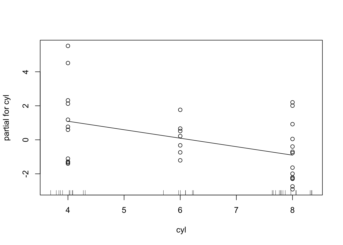
gam_model <- gam(mpg ~ s(wt) + s(hp) + cyl, data = mtcars)

# Model summary with significance tests
summary(gam_model)


Call: gam(formula = mpg ~ s(wt) + s(hp) + cyl, data = mtcars)
Deviance Residuals:
    Min      1Q  Median      3Q     Max 
-2.4914 -1.3267 -0.1171  0.9720  4.4302 

(Dispersion Parameter for gaussian family taken to be 4.5484)

    Null Deviance: 1126.047 on 31 degrees of freedom
Residual Deviance: 100.0641 on 22 degrees of freedom
AIC: 149.2945 

Number of Local Scoring Iterations: NA 

Anova for Parametric Effects
          Df Sum Sq Mean Sq  F value    Pr(>F)    
s(wt)      1 777.91  777.91 171.0300 7.491e-12 ***
s(hp)      1  97.78   97.78  21.4982 0.0001274 ***
cyl        1   5.16    5.16   1.1351 0.2982414    
Residuals 22 100.06    4.55                       
---
Signif. codes:  0 '***' 0.001 '**' 0.01 '*' 0.05 '.' 0.1 ' ' 1

Anova for Nonparametric Effects
            Npar Df Npar F  Pr(F)  
(Intercept)                        
s(wt)             3 2.4696 0.0887 .
s(hp)             3 2.0110 0.1418  
cyl                                
---
Signif. codes:  0 '***' 0.001 '**' 0.01 '*' 0.05 '.' 0.1 ' ' 1

Code

# Visualization of smooth terms
plot(gam_model, residuals = TRUE)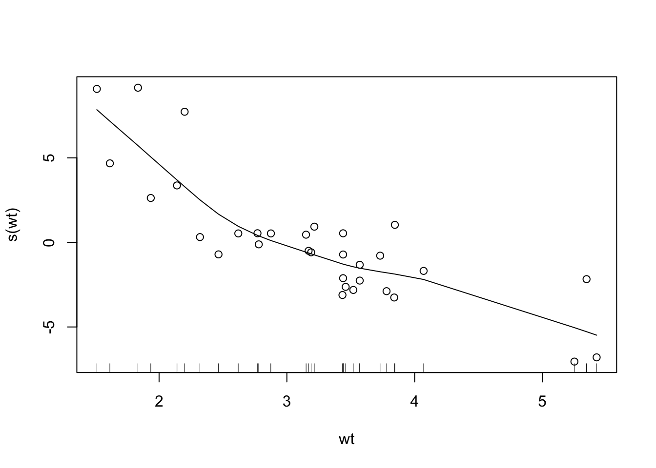

4 Ensemble Methods

4.1 Random Forests

R provides statistical random forest implementations:

Code

library(randomForest)

# Random forest with statistical output
rf_model <- randomForest(mpg ~ ., data = mtcars, importance = TRUE)

# Variable importance with statistical significance
importance(rf_model)

       %IncMSE IncNodePurity
cyl  11.937311     153.88376
disp 13.305115     256.59918
hp   12.549909     177.56688
drat  5.408634      54.53463
wt   12.802766     259.91706
qsec  3.994768      30.02724
vs    4.443471      34.22536
am    4.021616      28.26044
gear  3.555426      17.25570
carb  6.244602      38.54281

Code

varImpPlot(rf_model)

Code

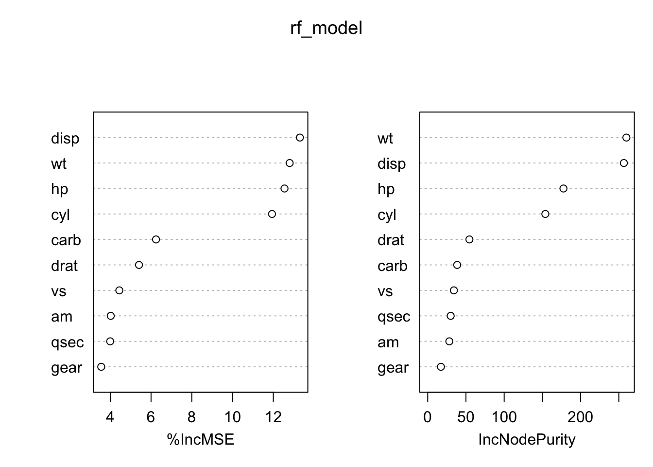
# Partial dependence plots
partialPlot(rf_model, mtcars, "wt")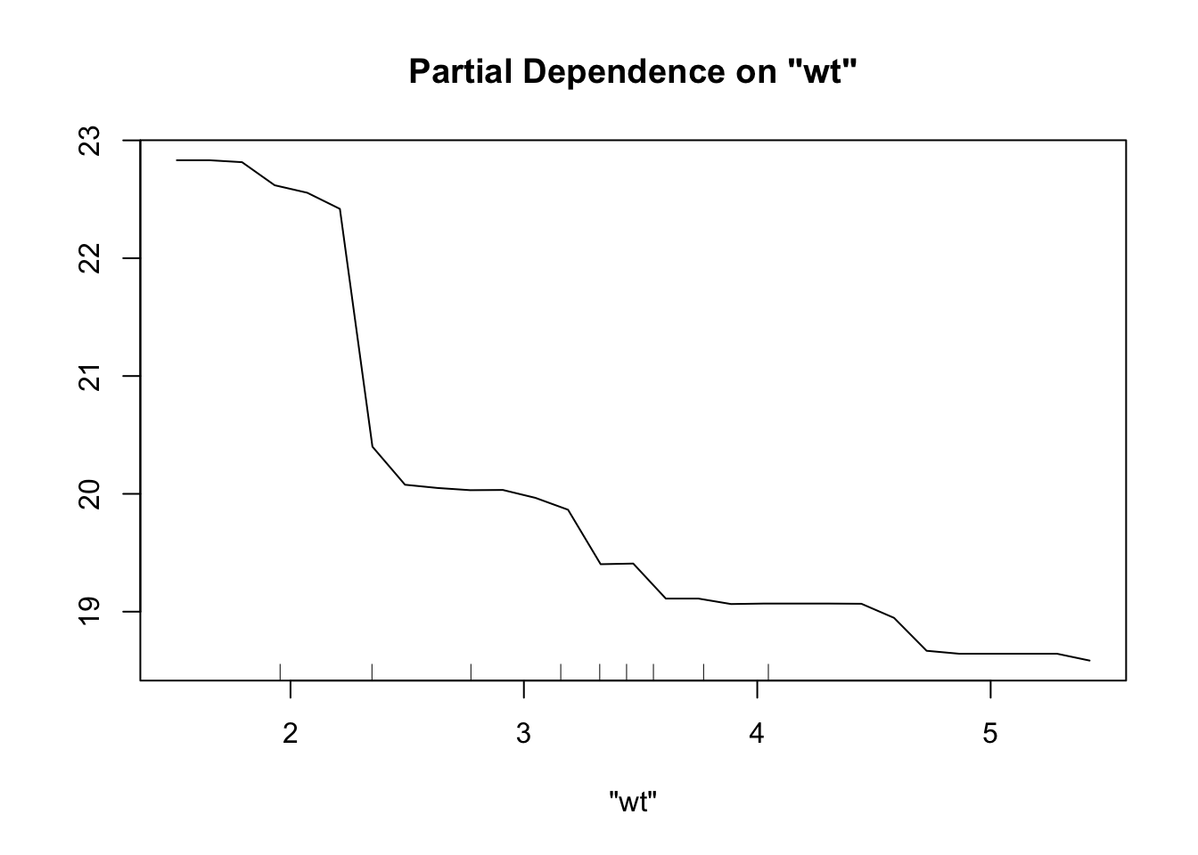

4.2 Gradient Boosting

R excels in statistical gradient boosting:

Code

library(gbm)

# Gradient boosting with statistical diagnostics
# Adjusted parameters for small dataset
gbm_model <- gbm(mpg ~ ., data = mtcars, 
                 distribution = "gaussian",
                 n.trees = 100,
                 interaction.depth = 2,
                 bag.fraction = 0.8,
                 n.minobsinnode = 3)

# Variable importance
summary(gbm_model)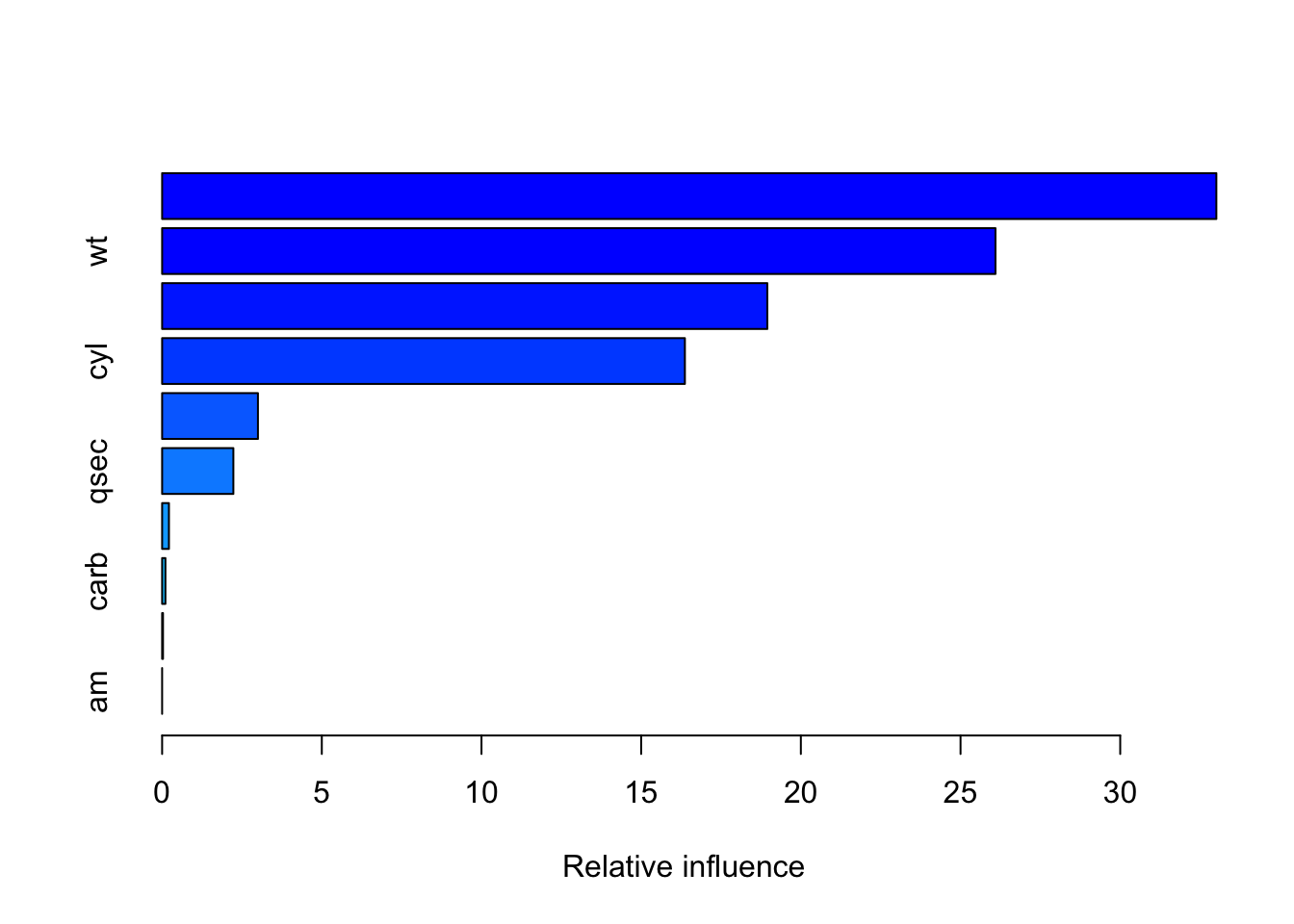

      var     rel.inf
hp     hp 33.01029394
wt     wt 26.09404675
disp disp 18.95097175
cyl   cyl 16.36905396
drat drat  3.00027174
qsec qsec  2.23090219
gear gear  0.21337593
carb carb  0.10342715
vs     vs  0.02765659
am     am  0.00000000

Code

# Partial dependence plots
plot(gbm_model, i.var = "wt")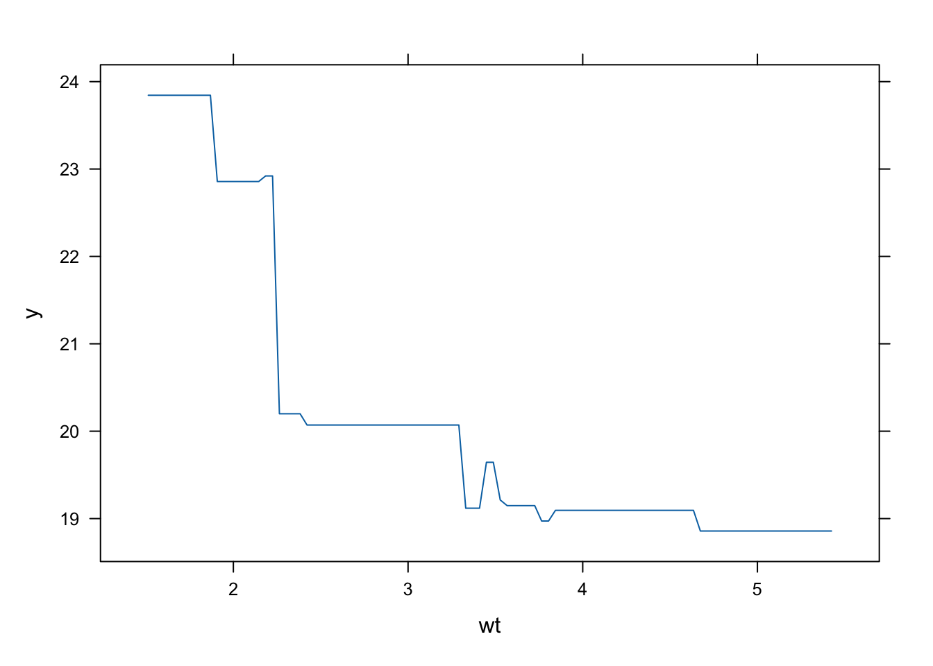

5 Model Diagnostics and Validation

5.1 Cross-Validation

R provides comprehensive validation tools:

Code

library(caret)
library(boot)

# Cross-validation with statistical rigor
cv_results <- cv.glm(mtcars, lm_model, K = 10)
cv_results$delta

[1] NaN NaN

Code

# Caret for systematic model comparison
control <- trainControl(method = "cv", number = 10)
model_comparison <- train(mpg ~ ., data = mtcars, 
                         method = "rf",
                         trControl = control)

5.2 Model Diagnostics

R excels in model diagnostics:

Code

# Comprehensive model diagnostics
library(car)

# Residual analysis
residualPlots(lm_model)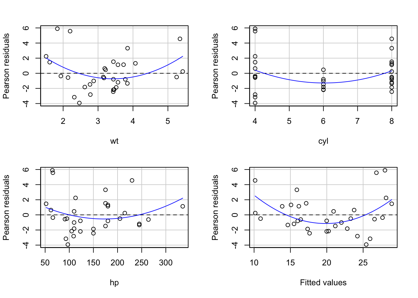

           Test stat Pr(>|Test stat|)   
wt            2.6276         0.014007 * 
cyl           1.6311         0.114476   
hp            1.8147         0.080701 . 
Tukey test    3.2103         0.001326 **
---
Signif. codes:  0 '***' 0.001 '**' 0.01 '*' 0.05 '.' 0.1 ' ' 1

Code

# Influence diagnostics
influencePlot(lm_model)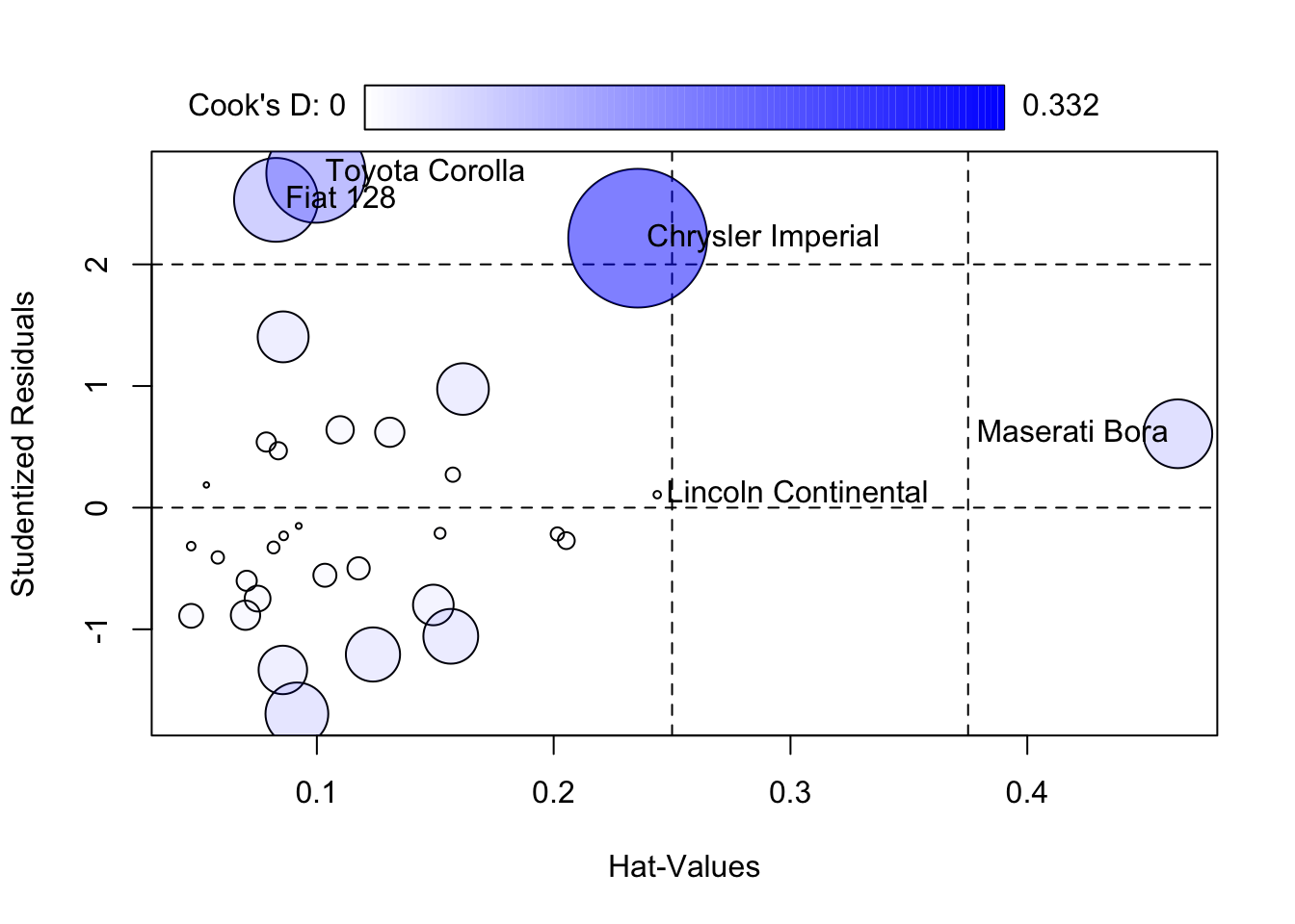

                      StudRes        Hat        CookD
Lincoln Continental 0.1065775 0.24373270 0.0009486833
Chrysler Imperial   2.2153833 0.23547715 0.3316313326
Fiat 128            2.5303244 0.08274176 0.1210330843
Toyota Corolla      2.7498370 0.09961207 0.1694339333
Maserati Bora       0.6073374 0.46356582 0.0815260489

Code

# Multicollinearity
vif(lm_model)

      wt      cyl       hp 
2.580486 4.757456 3.258481

Code

# Normality tests
shapiro.test(residuals(lm_model))


    Shapiro-Wilk normality test

data:  residuals(lm_model)
W = 0.93455, p-value = 0.05252

6 Bayesian Machine Learning

6.1 Bayesian Models

R provides sophisticated Bayesian ML:

Code

library(rstan)
library(brms)
library(rstanarm)

# Bayesian linear regression
bayes_model <- stan_glm(mpg ~ wt + cyl, data = mtcars,
                       family = gaussian(),
                       prior = normal(0, 10))


SAMPLING FOR MODEL 'continuous' NOW (CHAIN 1).
Chain 1: 
Chain 1: Gradient evaluation took 0.001327 seconds
Chain 1: 1000 transitions using 10 leapfrog steps per transition would take 13.27 seconds.
Chain 1: Adjust your expectations accordingly!
Chain 1: 
Chain 1: 
Chain 1: Iteration:    1 / 2000 [  0%]  (Warmup)
Chain 1: Iteration:  200 / 2000 [ 10%]  (Warmup)
Chain 1: Iteration:  400 / 2000 [ 20%]  (Warmup)
Chain 1: Iteration:  600 / 2000 [ 30%]  (Warmup)
Chain 1: Iteration:  800 / 2000 [ 40%]  (Warmup)
Chain 1: Iteration: 1000 / 2000 [ 50%]  (Warmup)
Chain 1: Iteration: 1001 / 2000 [ 50%]  (Sampling)
Chain 1: Iteration: 1200 / 2000 [ 60%]  (Sampling)
Chain 1: Iteration: 1400 / 2000 [ 70%]  (Sampling)
Chain 1: Iteration: 1600 / 2000 [ 80%]  (Sampling)
Chain 1: Iteration: 1800 / 2000 [ 90%]  (Sampling)
Chain 1: Iteration: 2000 / 2000 [100%]  (Sampling)
Chain 1: 
Chain 1:  Elapsed Time: 0.023 seconds (Warm-up)
Chain 1:                0.025 seconds (Sampling)
Chain 1:                0.048 seconds (Total)
Chain 1: 

SAMPLING FOR MODEL 'continuous' NOW (CHAIN 2).
Chain 2: 
Chain 2: Gradient evaluation took 6e-06 seconds
Chain 2: 1000 transitions using 10 leapfrog steps per transition would take 0.06 seconds.
Chain 2: Adjust your expectations accordingly!
Chain 2: 
Chain 2: 
Chain 2: Iteration:    1 / 2000 [  0%]  (Warmup)
Chain 2: Iteration:  200 / 2000 [ 10%]  (Warmup)
Chain 2: Iteration:  400 / 2000 [ 20%]  (Warmup)
Chain 2: Iteration:  600 / 2000 [ 30%]  (Warmup)
Chain 2: Iteration:  800 / 2000 [ 40%]  (Warmup)
Chain 2: Iteration: 1000 / 2000 [ 50%]  (Warmup)
Chain 2: Iteration: 1001 / 2000 [ 50%]  (Sampling)
Chain 2: Iteration: 1200 / 2000 [ 60%]  (Sampling)
Chain 2: Iteration: 1400 / 2000 [ 70%]  (Sampling)
Chain 2: Iteration: 1600 / 2000 [ 80%]  (Sampling)
Chain 2: Iteration: 1800 / 2000 [ 90%]  (Sampling)
Chain 2: Iteration: 2000 / 2000 [100%]  (Sampling)
Chain 2: 
Chain 2:  Elapsed Time: 0.024 seconds (Warm-up)
Chain 2:                0.023 seconds (Sampling)
Chain 2:                0.047 seconds (Total)
Chain 2: 

SAMPLING FOR MODEL 'continuous' NOW (CHAIN 3).
Chain 3: 
Chain 3: Gradient evaluation took 6e-06 seconds
Chain 3: 1000 transitions using 10 leapfrog steps per transition would take 0.06 seconds.
Chain 3: Adjust your expectations accordingly!
Chain 3: 
Chain 3: 
Chain 3: Iteration:    1 / 2000 [  0%]  (Warmup)
Chain 3: Iteration:  200 / 2000 [ 10%]  (Warmup)
Chain 3: Iteration:  400 / 2000 [ 20%]  (Warmup)
Chain 3: Iteration:  600 / 2000 [ 30%]  (Warmup)
Chain 3: Iteration:  800 / 2000 [ 40%]  (Warmup)
Chain 3: Iteration: 1000 / 2000 [ 50%]  (Warmup)
Chain 3: Iteration: 1001 / 2000 [ 50%]  (Sampling)
Chain 3: Iteration: 1200 / 2000 [ 60%]  (Sampling)
Chain 3: Iteration: 1400 / 2000 [ 70%]  (Sampling)
Chain 3: Iteration: 1600 / 2000 [ 80%]  (Sampling)
Chain 3: Iteration: 1800 / 2000 [ 90%]  (Sampling)
Chain 3: Iteration: 2000 / 2000 [100%]  (Sampling)
Chain 3: 
Chain 3:  Elapsed Time: 0.024 seconds (Warm-up)
Chain 3:                0.025 seconds (Sampling)
Chain 3:                0.049 seconds (Total)
Chain 3: 

SAMPLING FOR MODEL 'continuous' NOW (CHAIN 4).
Chain 4: 
Chain 4: Gradient evaluation took 3e-06 seconds
Chain 4: 1000 transitions using 10 leapfrog steps per transition would take 0.03 seconds.
Chain 4: Adjust your expectations accordingly!
Chain 4: 
Chain 4: 
Chain 4: Iteration:    1 / 2000 [  0%]  (Warmup)
Chain 4: Iteration:  200 / 2000 [ 10%]  (Warmup)
Chain 4: Iteration:  400 / 2000 [ 20%]  (Warmup)
Chain 4: Iteration:  600 / 2000 [ 30%]  (Warmup)
Chain 4: Iteration:  800 / 2000 [ 40%]  (Warmup)
Chain 4: Iteration: 1000 / 2000 [ 50%]  (Warmup)
Chain 4: Iteration: 1001 / 2000 [ 50%]  (Sampling)
Chain 4: Iteration: 1200 / 2000 [ 60%]  (Sampling)
Chain 4: Iteration: 1400 / 2000 [ 70%]  (Sampling)
Chain 4: Iteration: 1600 / 2000 [ 80%]  (Sampling)
Chain 4: Iteration: 1800 / 2000 [ 90%]  (Sampling)
Chain 4: Iteration: 2000 / 2000 [100%]  (Sampling)
Chain 4: 
Chain 4:  Elapsed Time: 0.024 seconds (Warm-up)
Chain 4:                0.022 seconds (Sampling)
Chain 4:                0.046 seconds (Total)
Chain 4:

Code

# Posterior analysis
posterior_interval(bayes_model)

                   5%        95%
(Intercept) 36.832343 42.5697902
wt          -4.508066 -1.8619240
cyl         -2.248036 -0.7854588
sigma        2.127666  3.3044072

Code

plot(bayes_model)

6.2 Probabilistic Programming

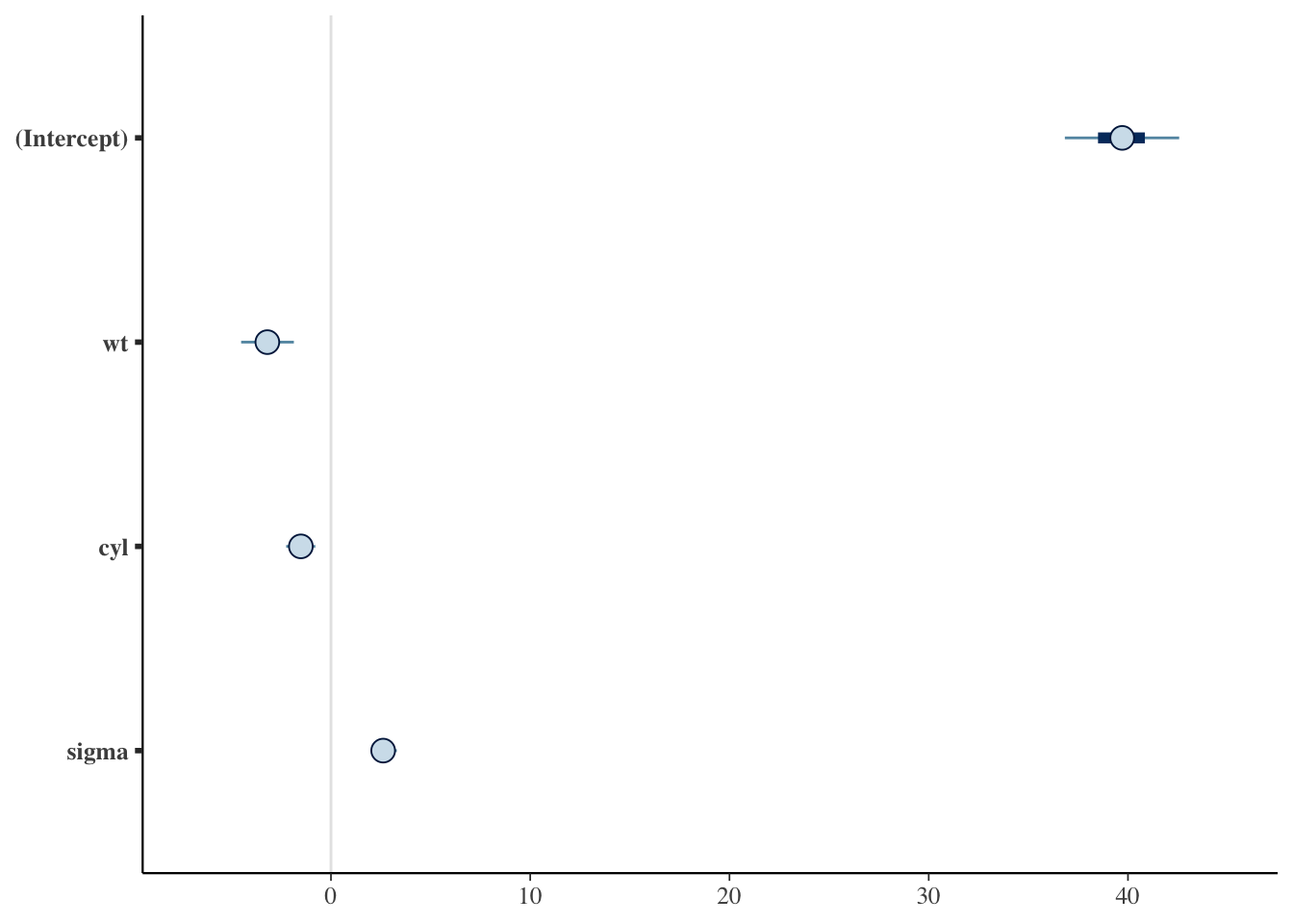
R excels in probabilistic programming:

Code

# Stan integration for complex models
# - Hierarchical models
# - Time series models
# - Spatial models
# - Custom likelihoods
# - Advanced inference

7 Interpretable Machine Learning

7.1 Model Interpretability

R emphasizes model interpretability:

Code

library(iml)
library(DALEX)

# Model interpretability tools
# - Partial dependence plots
# - Individual conditional expectation
# - Feature importance
# - Model explanations
# - Fairness analysis

7.2 Explainable AI

R provides explainable AI tools:

Code

# Explainable AI capabilities
# - LIME implementation
# - SHAP values
# - Model-agnostic explanations
# - Feature interactions
# - Decision paths

8 Python’s ML Limitations

8.1 Engineering Focus

Python’s ML is engineering-focused:

# Python ML emphasizes:
# - Scalability
# - Production deployment
# - Deep learning
# - Engineering efficiency
# - Less statistical rigor

8.2 Limited Statistical Depth

Python lacks statistical depth:

# Python has limited:
# - Statistical diagnostics
# - Model interpretability
# - Uncertainty quantification
# - Research reproducibility
# - Academic validation

9 Performance Comparison

Feature	R	Python
Statistical Foundation	Excellent	Limited
Model Diagnostics	Comprehensive	Basic
Interpretability	Advanced	Limited
Research Integration	Strong	Weak
Uncertainty Quantification	Sophisticated	Basic
Academic Validation	Peer-reviewed	Variable
Deep Learning	Limited	Excellent
Production Deployment	Limited	Excellent

10 Key Advantages of R for ML

10.1 1. Statistical Rigor

Code

# R ensures statistical rigor in ML:
# - Proper model diagnostics
# - Uncertainty quantification
# - Statistical significance testing
# - Model validation
# - Research reproducibility

10.2 2. Interpretability Focus

Code

# R emphasizes interpretability:
# - Model explanations
# - Feature importance
# - Partial dependence plots
# - Statistical inference
# - Research transparency

10.3 3. Research Integration

Code

# R's ML packages are:
# - Peer-reviewed
# - Published in journals
# - Used in research
# - Well-documented
# - Statistically validated

11 Complementary Approaches

11.1 R + Python Integration

R and Python can complement each other:

Code

# R for:
# - Statistical modeling
# - Model diagnostics
# - Research validation
# - Interpretability
# - Academic publishing

# Python for:
# - Deep learning
# - Production deployment
# - Large-scale processing
# - Engineering workflows
# - Web applications

11.2 Best of Both Worlds

Code

# Optimal workflow:
# 1. R for exploratory analysis and statistical modeling
# 2. Python for deep learning and production deployment
# 3. R for model interpretation and validation
# 4. Python for scaling and deployment

12 Conclusion

R’s machine learning approach provides:

Statistical rigor and model diagnostics
Research-grade implementations with peer review
Emphasis on interpretability and transparency
Comprehensive validation and uncertainty quantification
Academic integration and reproducibility
Complementary strengths to Python’s engineering focus

While Python excels in deep learning and production deployment, R provides unique advantages for statistical machine learning, research, and interpretable AI applications.

This concludes our series on “R Beats Python” - exploring the specific areas where R provides superior capabilities for data science and statistical analysis.