Statistical Modeling: Why R Outperforms Python

statistics

modeling

comparison

A deep dive into R’s superior statistical modeling capabilities, from GLMs to mixed models

Published

June 26, 2025

1 Introduction

When it comes to statistical modeling, R was built from the ground up for this purpose. While Python has made significant strides with libraries like statsmodels and scipy.stats, R’s statistical ecosystem remains unmatched in depth, breadth, and ease of use.

2 Generalized Linear Models (GLMs)

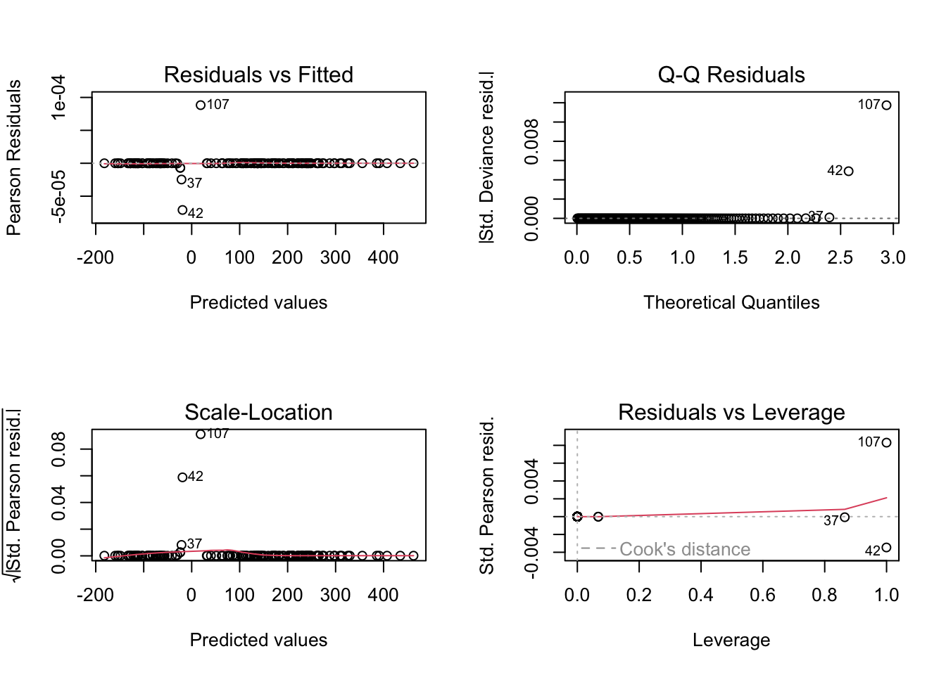
2.1 R Approach

Code

# Load required libraries
library(stats)

# Fit a logistic regression model
model_r <- glm(Species ~ Sepal.Length + Sepal.Width, 
               data = iris, 
               family = binomial(link = "logit"))

# Comprehensive model summary
summary(model_r)


Call:
glm(formula = Species ~ Sepal.Length + Sepal.Width, family = binomial(link = "logit"), 
    data = iris)

Coefficients:
             Estimate Std. Error z value Pr(>|z|)
(Intercept)    -437.2   128737.9  -0.003    0.997
Sepal.Length    163.4    45394.8   0.004    0.997
Sepal.Width    -137.9    44846.1  -0.003    0.998

(Dispersion parameter for binomial family taken to be 1)

    Null deviance: 1.9095e+02  on 149  degrees of freedom
Residual deviance: 2.7060e-08  on 147  degrees of freedom
AIC: 6

Number of Fisher Scoring iterations: 25

Code

# Diagnostic plots
par(mfrow = c(2, 2))
plot(model_r)

2.2 Python Approach

import pandas as pd
import statsmodels.api as sm
from sklearn.linear_model import LogisticRegression

# Fit logistic regression
X = iris[['sepal_length', 'sepal_width']]
y = (iris['species'] == 'setosa').astype(int)

# Using statsmodels
model_py = sm.GLM(y, sm.add_constant(X), family=sm.families.Binomial())
result = model_py.fit()
print(result.summary())

# Diagnostic plots require additional work
import matplotlib.pyplot as plt
import seaborn as sns

3 Mixed Effects Models

3.1 R’s Superior Implementation

Code

library(lme4)

# Fit a mixed effects model
mixed_model <- lmer(Reaction ~ Days + (1 + Days | Subject), 
                    data = sleepstudy)

# Comprehensive output
summary(mixed_model)

Linear mixed model fit by REML ['lmerMod']
Formula: Reaction ~ Days + (1 + Days | Subject)
   Data: sleepstudy

REML criterion at convergence: 1743.6

Scaled residuals: 
    Min      1Q  Median      3Q     Max 
-3.9536 -0.4634  0.0231  0.4634  5.1793 

Random effects:
 Groups   Name        Variance Std.Dev. Corr
 Subject  (Intercept) 612.10   24.741       
          Days         35.07    5.922   0.07
 Residual             654.94   25.592       
Number of obs: 180, groups:  Subject, 18

Fixed effects:
            Estimate Std. Error t value
(Intercept)  251.405      6.825  36.838
Days          10.467      1.546   6.771

Correlation of Fixed Effects:
     (Intr)
Days -0.138

Code

# Random effects
ranef(mixed_model)

$Subject
    (Intercept)        Days
308   2.2585509   9.1989758
309 -40.3987381  -8.6196806
310 -38.9604090  -5.4488565
330  23.6906196  -4.8143503
331  22.2603126  -3.0699116
332   9.0395679  -0.2721770
333  16.8405086  -0.2236361
334  -7.2326151   1.0745816
335  -0.3336684 -10.7521652
337  34.8904868   8.6282652
349 -25.2102286   1.1734322
350 -13.0700342   6.6142178
351   4.5778642  -3.0152621
352  20.8636782   3.5360011
369   3.2754656   0.8722149
370 -25.6129993   4.8224850
371   0.8070461  -0.9881562
372  12.3145921   1.2840221

with conditional variances for "Subject"

Code

# Model diagnostics
plot(mixed_model)

3.2 Python’s Limited Options

# Python has limited mixed effects support
import statsmodels.api as sm
from statsmodels.regression.mixed_linear_model import MixedLM

# Much more complex syntax and limited functionality
# No equivalent to lme4's comprehensive output

4 Time Series Analysis

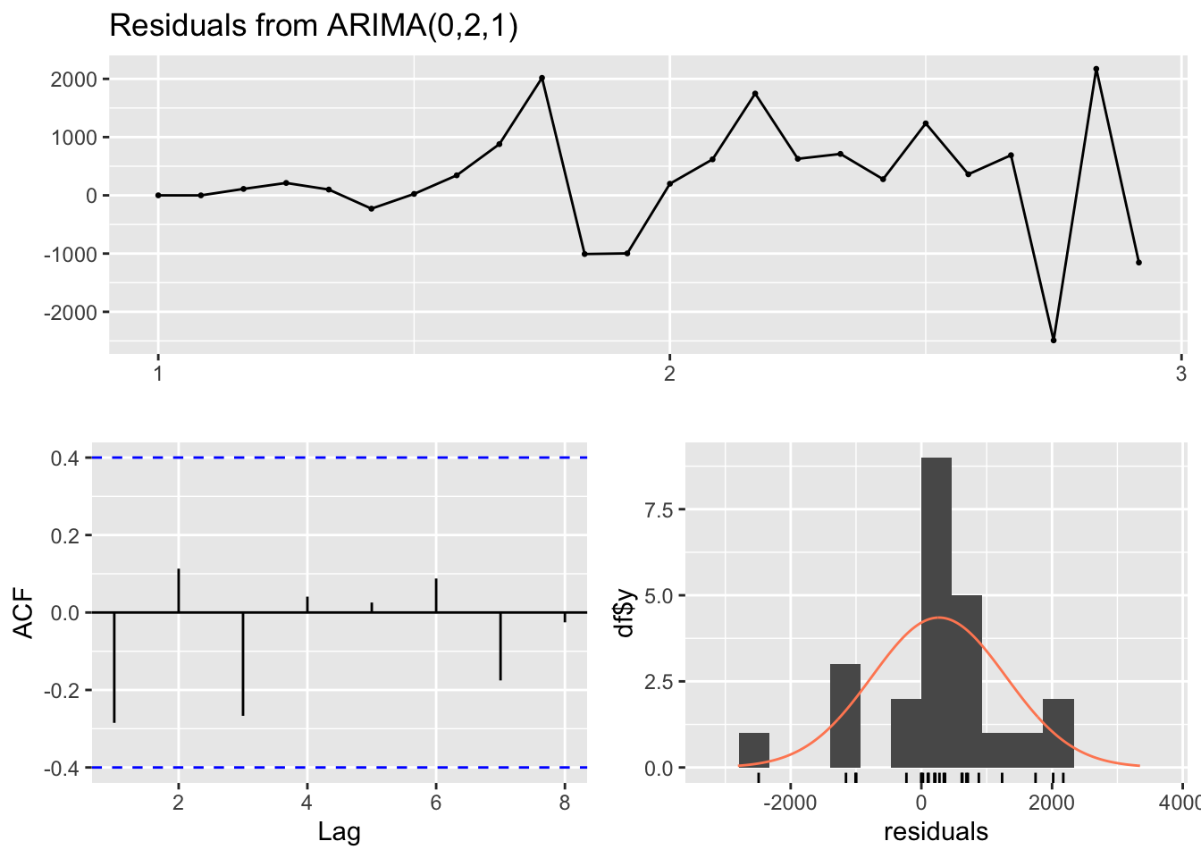
4.1 R’s Time Series Ecosystem

Code

library(forecast)
library(tseries)

# Fit ARIMA model
ts_data <- ts(airmiles, frequency = 12)
arima_model <- auto.arima(ts_data)

# Comprehensive diagnostics
checkresiduals(arima_model)


    Ljung-Box test

data:  Residuals from ARIMA(0,2,1)
Q* = 4.7529, df = 4, p-value = 0.3136

Model df: 1.   Total lags used: 5

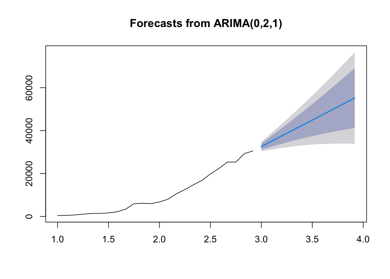
Code

# Forecasting
forecast_result <- forecast(arima_model, h = 12)
plot(forecast_result)

4.2 Python’s Fragmented Approach

from statsmodels.tsa.arima.model import ARIMA
from statsmodels.tsa.stattools import adfuller

# More complex setup required
# Limited diagnostic tools
# Separate packages needed for different functionality

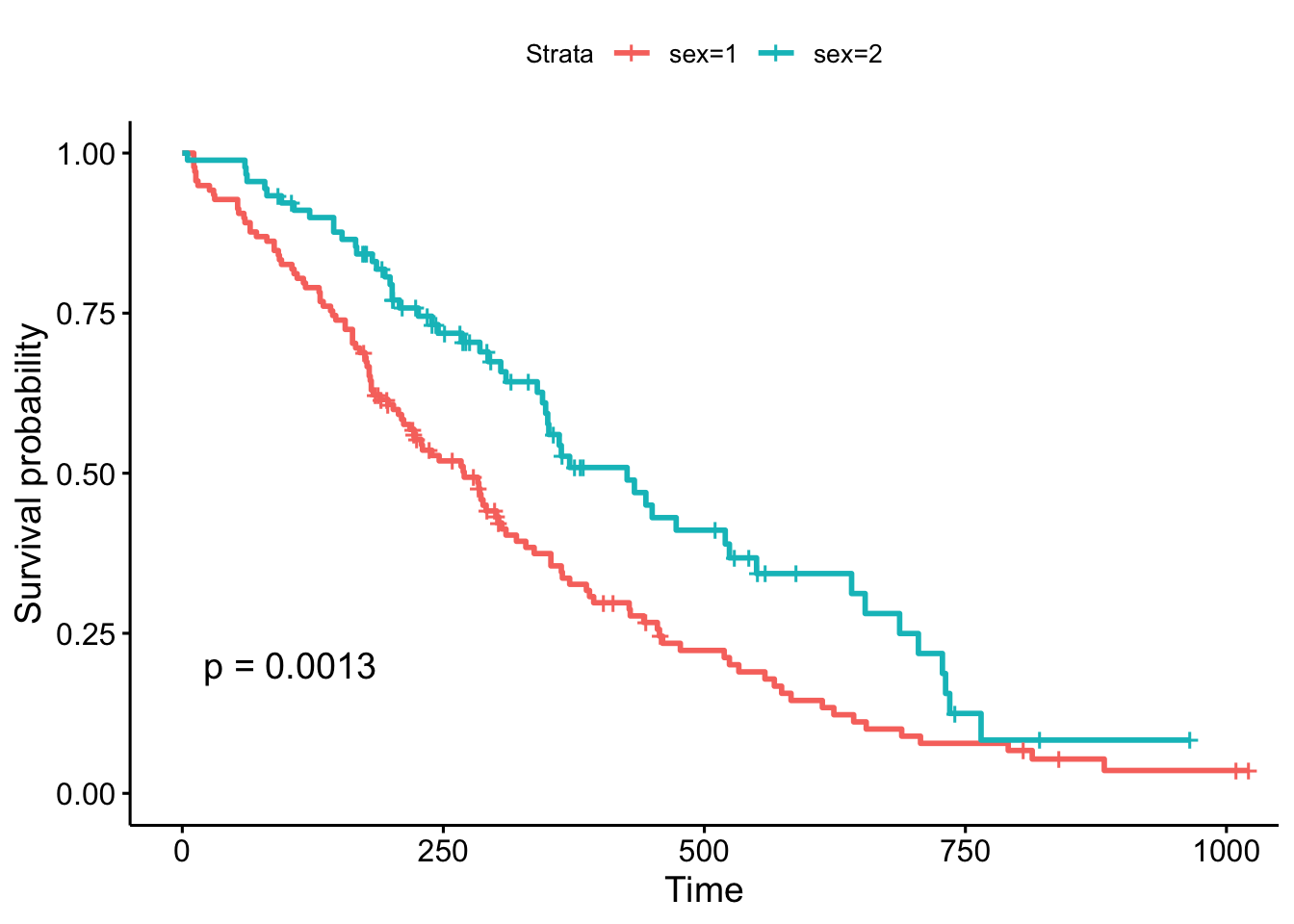
5 Survival Analysis

5.1 R’s Comprehensive Survival Tools

Code

library(survival)
library(survminer)

# Fit Cox proportional hazards model
cox_model <- coxph(Surv(time, status) ~ age + sex + ph.ecog, 
                   data = lung)

# Comprehensive output
summary(cox_model)

Call:
coxph(formula = Surv(time, status) ~ age + sex + ph.ecog, data = lung)

  n= 227, number of events= 164 
   (1 observation deleted due to missingness)

             coef exp(coef)  se(coef)      z Pr(>|z|)    
age      0.011067  1.011128  0.009267  1.194 0.232416    
sex     -0.552612  0.575445  0.167739 -3.294 0.000986 ***
ph.ecog  0.463728  1.589991  0.113577  4.083 4.45e-05 ***
---
Signif. codes:  0 '***' 0.001 '**' 0.01 '*' 0.05 '.' 0.1 ' ' 1

        exp(coef) exp(-coef) lower .95 upper .95
age        1.0111     0.9890    0.9929    1.0297
sex        0.5754     1.7378    0.4142    0.7994
ph.ecog    1.5900     0.6289    1.2727    1.9864

Concordance= 0.637  (se = 0.025 )
Likelihood ratio test= 30.5  on 3 df,   p=1e-06
Wald test            = 29.93  on 3 df,   p=1e-06
Score (logrank) test = 30.5  on 3 df,   p=1e-06

Code

# Survival curves
fit <- survfit(Surv(time, status) ~ sex, data = lung)
ggsurvplot(fit, data = lung, pval = TRUE)

5.2 Python’s Limited Survival Analysis

# Python has very limited survival analysis capabilities
# Most implementations are basic or require external packages
# No equivalent to R's comprehensive survival analysis ecosystem

6 Key Advantages of R for Statistical Modeling

6.1 1. Built-in Statistical Functions

R provides comprehensive statistical functions out of the box:

Code

# T-test with detailed output
t.test(extra ~ group, data = sleep)


    Welch Two Sample t-test

data:  extra by group
t = -1.8608, df = 17.776, p-value = 0.07939
alternative hypothesis: true difference in means between group 1 and group 2 is not equal to 0
95 percent confidence interval:
 -3.3654832  0.2054832
sample estimates:
mean in group 1 mean in group 2 
           0.75            2.33

Code

# ANOVA with post-hoc tests
aov_result <- aov(weight ~ group, data = PlantGrowth)
TukeyHSD(aov_result)

  Tukey multiple comparisons of means
    95% family-wise confidence level

Fit: aov(formula = weight ~ group, data = PlantGrowth)

$group
            diff        lwr       upr     p adj
trt1-ctrl -0.371 -1.0622161 0.3202161 0.3908711
trt2-ctrl  0.494 -0.1972161 1.1852161 0.1979960
trt2-trt1  0.865  0.1737839 1.5562161 0.0120064

Code

# Correlation with significance testing
cor.test(mtcars$mpg, mtcars$wt, method = "pearson")


    Pearson's product-moment correlation

data:  mtcars$mpg and mtcars$wt
t = -9.559, df = 30, p-value = 1.294e-10
alternative hypothesis: true correlation is not equal to 0
95 percent confidence interval:
 -0.9338264 -0.7440872
sample estimates:
       cor 
-0.8676594

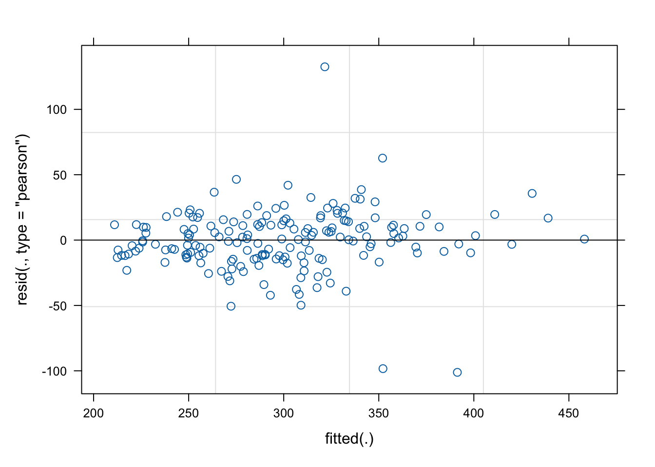
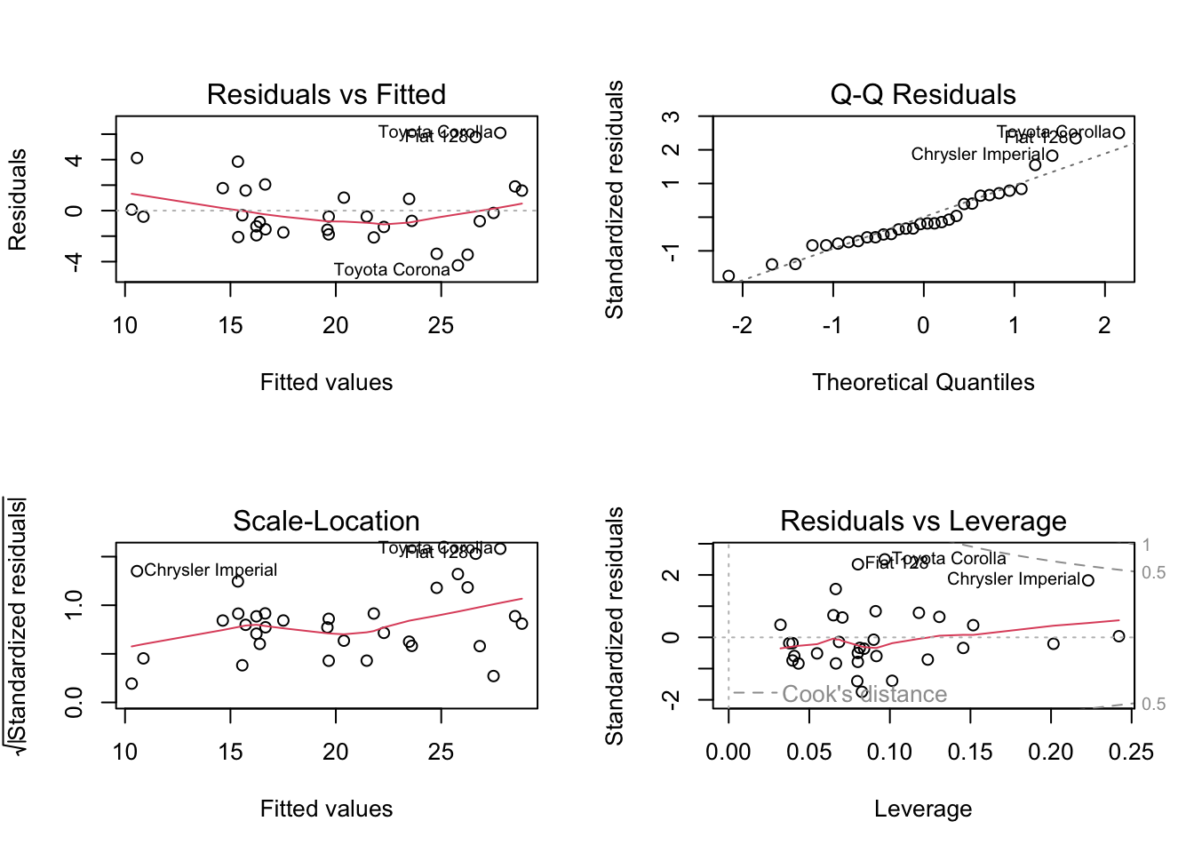
6.2 2. Comprehensive Model Diagnostics

R provides extensive diagnostic tools:

Code

# Model diagnostics for linear regression
lm_model <- lm(mpg ~ wt + cyl, data = mtcars)

# Comprehensive diagnostic plots
par(mfrow = c(2, 2))
plot(lm_model)

Code

# Additional diagnostics
library(car)
vif(lm_model)  # Variance inflation factors

      wt      cyl 
2.579312 2.579312

Code

durbinWatsonTest(lm_model)  # Autocorrelation test

 lag Autocorrelation D-W Statistic p-value
   1       0.1302185      1.671096   0.286
 Alternative hypothesis: rho != 0

6.3 3. Advanced Statistical Packages

R’s CRAN repository hosts specialized statistical packages:

nlme: Nonlinear mixed effects models
mgcv: Generalized additive models
brms: Bayesian regression models
rstan: Stan integration for Bayesian analysis

7 Performance Comparison

Feature	R	Python
GLM Implementation	Native, comprehensive	Basic, requires statsmodels
Mixed Effects	lme4, nlme	Limited options
Time Series	forecast, tseries	Fragmented ecosystem
Survival Analysis	survival, survminer	Very limited
Model Diagnostics	Built-in, extensive	Basic, requires work
Statistical Tests	Comprehensive	Basic

8 Conclusion

For statistical modeling, R provides:

Native statistical capabilities built into the language
Comprehensive model diagnostics and validation tools
Extensive package ecosystem for specialized analyses
Better statistical output with publication-ready results
Easier syntax for statistical operations

While Python excels in machine learning and general programming, R remains the superior choice for traditional statistical modeling, especially in research and academic settings.

Next: Data Visualization: R’s ggplot2 vs Python’s matplotlib